Last week we setup our simulation domain, ability to represent particles on screen and even integrate their position over time.

I hope you enjoyed the official launch (click here if you missed that)!

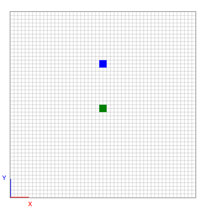
Not bad for a few days of work, I’d say!

Before we steam ahead, I want to cover some of the concepts that allow this to happen (it will also help us later on in the project).

What is this stuff made of?

It’s important to note: when we use FEA and CFD tools as Engineers, we’re usually interested in the macro-scale behaviour of a solid or fluid.

A tonne of simulation modelling methods have been developed over the last few decades, each with their own advantages and disadvantages.

The most common are mesh or particle-based methods.

Namely, FEA tools usually represent solids by arranging connected nodes, allowing the resulting forces to be tracked across the individual positions as the mesh deforms. This is known as a Lagrangian format.

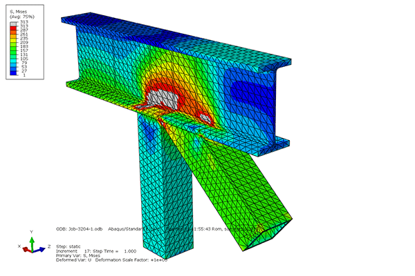
The output is material stress, strain and displacement.

CFD tools most commonly represent fluids using a static mesh which will allow the fluid to move through it based on the cell properties at a given location. OpenFOAM is an example of this.

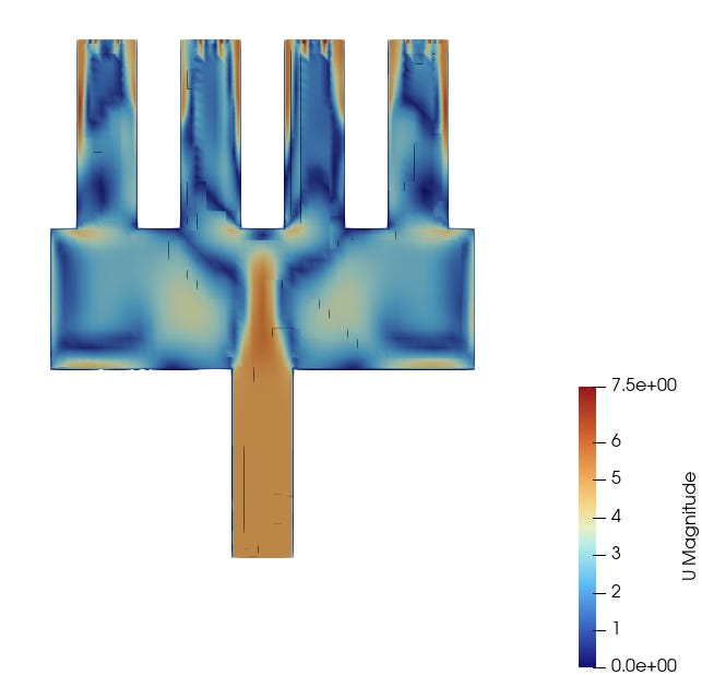
The output is fluid velocity, pressure and flow trajectories.

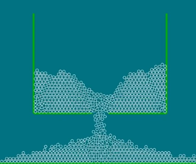
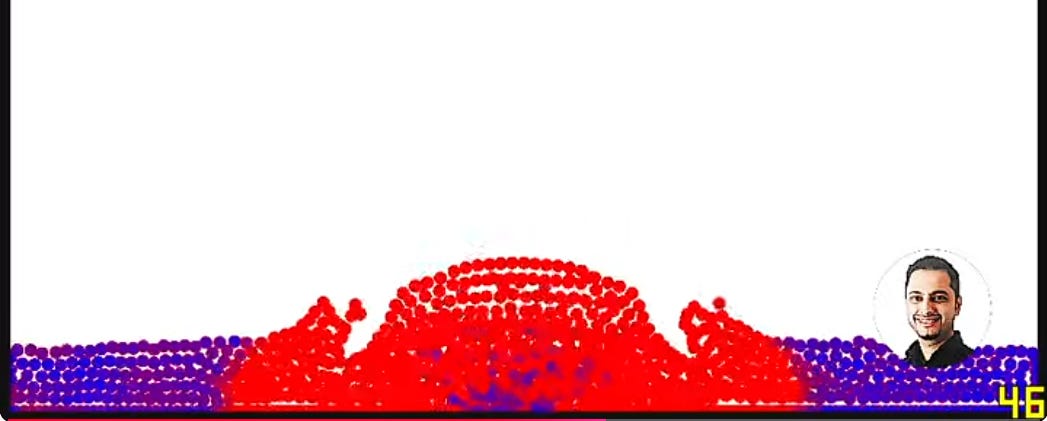
To capture large deformations, splashing or mixing behaviour, say the fluids in a gearbox or engine etc.

I actually developed these types of tools in the past (both available to watch on my YouTube channel):

What have we modelled so far?

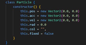
Our current code models implements the individual particles in an X-Y vector space. It’s closer to a DEM particle implementation right now, but we’ll soon turn it into an FEM then FVM-style model.

As long as it keeps within the scope of the project – building an intuitive understanding of fluid dynamics and how to use these tools effectively.

This is how intuition is best built. Trust me. it’s well worth it!

We currently have:

• positions for current locations

• velocities to calculate their new locations

• accelerations to feed into the velocities

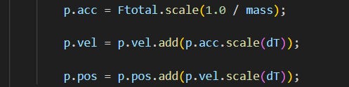
• forces that act on the accelerations

• an integration loop which approximates the future positions of particles

Let’s setup a solid model.

What is a solid anyway? And how is a fluid different?

These are very important questions in our quest to develop an intuition for fluid dynamics.

The concept of a fluid shapes everything here.

A solid is tightly packed (most dense) with very strong inter-molecular forces at play.

A fluid actually exists in two forms: a Liquid and a Gas.

A liquid is densely packed, with strong cohesive forces and maintains volume. They can form a free surface which is affected by gravitational fields.

Gas is less dense with weak cohesive forces and it can’t form a free surface.
The molecules fill all available space.

Physics covers a wide range of problems – descriptions and equations are actually statements pertaining to a specific scenario.

I agree, that was a mouthful!

Before we model it, we typically need to make some statements and assumptions.

• What arrangement does a solid have?
  We’re assuming a densely-packed structure.

• Where will the Shear Force be applied?

  To the side of the structure, with the Frictional force of the floor acting against it.

• Will material deform? How is it expected to do so?

  There’ll be shear stress profile experienced under load, varying depending on the particle location being sampled.

• What happens when you stop applying the Force(s)?
  The structure will resume it’s previous, no-load configuration. Upper particles should try moving in the F direction, but bonds should resist.

All this before any computational model has been created.

Note, most of this has come from reflection and theoretical science we meet at high school.

Watch me talk and walk you through this:

The takeaway.

It’s important to realise that our model has a number of properties:

• A Stiffness – resistance to deformation

• A Mass – resistance to acceleration

• A Damping – dissipation of energy

And you can see it all, right before your eyes!

Ah, the power of visualisation creates an intuition hard to get from textbooks alone.

Don’t you think every Engineer should have access to a model like this in their back pocket?!

I do.

Have a great week!
Nasser