
If you’re new here, welcome! 🙌
I’m Nasser, an ex-Senior Mechanical Engineer turned Engineering Software Developer, sharing clear explanations with deep insights from my lived experience in fast-moving tech industries.
If you find this post helpful and / or insightful, then consider supporting me directly.
Upgrade to paid and access premium resources.
I’ve always been interested in the little details that makes things work as an Engineer.
This has always really been true for me.
High-accuracy CFD solvers often need a gazillion-cell mesh, but it’s a single cell with neighbours that holds the key to how they work.

Last week I calculated the heat flux from the gradient, then heat transfer rate from this flux.
From this, the net cell balance (what goes in and what goes out) can be calculated…
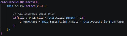
From here the scalar (Temperature in this case) is updated as required.
With a zero net transfer balance, the configuration is actually a steady state distribution.
In other words… “Nothing is created. Nothing is Lost.”
It’s all in the name of conservation.
And it’s the heart of the Finite Volume Method (FVM).
Whilst it’s a straight-forward calculation, it’s often difficult to see or appreciate when you look at the theory or open-source numerical codebases.
That’s why I’m determined to “strip things back”.
I want you to see what I see.
What does ‘fixedGradient’ in OpenFOAM really mean?!
If you we’re looking closely at the code snippet above, you’d have seen that we access the internal cells of the mesh (1 through to 8).
The reason is that we have no cell to the left of cell 0, nor any to the right of cell 9.
These can be referred to as the boundary cells, as marked in my code.
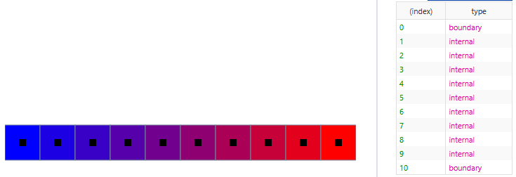
From this point, I can artificially impose a boundary condition by setting the gradient of the end cells to a fixed temperature, resulting in the heat flux being the same as the internal cells.
This results in net-zero heat transfer at the boundary cells.
And it’s exactly how OpenFOAM behaves when you type ‘fixedGradient’ for a boundary wall in the 0/ directory!
Now you know.
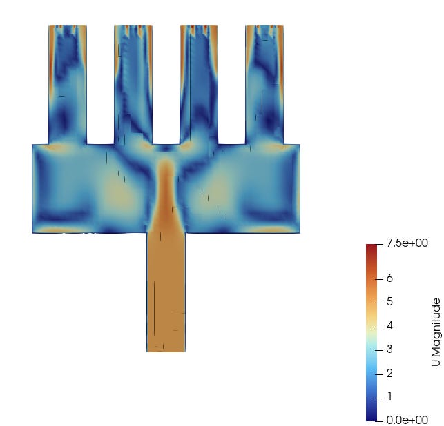
In fact there are many other direct connections with OpenFOAM.
-
The mesh contains points, faces, cells and their connectivity.
This is useful to know since you can start inspecting the mesh like a doctor inspects the body – they know what should be there and how it’s connected! -
OpenFOAM must approximate from values stored on the mesh.
Do you know that thegradSchemessection in fvSchemes determines how gradients are calculated? Well, I’ve just made it visual! -
Conservation happens at the faces.
Mass flowing out of one cell must enter a neighbouring one or be set a boundary condition to ensure correct calculations. -
Every calculation is done sequentially.
Updates are performed per time-step in a continuous loop. -
Numerical results need to be validated.
Convergence isn’t enough, seriously. That’s why I always use integrated field values.
What we’ve really done here.
Our code currently calculates the gradient between cells in the given time step.
It then uses that to model the diffusion of heat (our scalar field).
Honestly, don’t make it more complex than this.
Soon, I’ll implement convection allowing us to look at the behaviour of fluid being transported along geometry.
Neat!
Unfortunately, I didn’t get a change to create a video this week, but I intend to create a longer and detailed one soon, most likely including fresh updates to the code!
😎 Interesting things from around the web I found this week:
-
A curated list of repositories related to fluid dynamics. Lots of Python and C++ libraries and shared resources:
-
Interactive simulations you can play with around physics concepts:
https://ophysics.com/fl.html -
Manchester University here in the UK has an incredible overview of the various fields within Fluid Dynamics and industrial applications:
https://www.masc.manchester.ac.uk/research/
As always, don’t forget to watch and subscribe to my YouTube channel – it’s growing steadily, thanks to the community.
🎥 https://youtube.com/@nasserm_engineer?si=Qj1x7QBfzrhnbxQb
Have a great week!
Nasser
