
If you’re new here, welcome! 🙌
I’m Nasser, an ex Senior Mechanical Engineer turned Engineering Software Developer. I’m obsessed with making physics solvers and simulation technology easier to understand for Engineers and Researchers, through my personal experience and unique perspective. Understanding these tools beyond the GUI changed my Engineering career forever.
🎥 A video accompanies this post (towards the end).
Turning theory into a practical implementation was always going to be challenging, even when you “get it”.
After all this is what happens in organised / academic research too!
Over the past week I’ve been busy refactoring the code we have so far in preparation to go from an understanding of solid behaviour to modelling the motion of fluids.
If you missed any of the previous posts in this series, catch up here:
From solids to fluids.
As mentioned previously, we know that fluids cannot resist deforming under any amount of shear stress.
(It just means the molecules within the fluid readily slide across each other).

The theory behind this is governed by the following physics:
-
A conservation of mass.
-
A conservation of momentum.
-
A conservation of energy.
Nothing is being created (adding to) or lost (subtracting from).
Basically everything is accounted for.
A bunch of particles fails to do this type of conservation justice, mainly for two reasons – the challenges in smoothing particle interactions and the frustration in managing boundary conditions.
From particles to grids.
When modelling a fluid, CFD solvers need a mesh – a grid of cells that define the geometry in 3D space (X, Y, Z).
Specifically, this is the Eulerian view of the world.
We’re taking fixed locations in space and allowing fluid to flow past them.
So when you import and load a 3D CAD model into a CFD tool, the first step is to generate a mesh.
For the purpose of our project, the mesh at this stage is simply a set of 10 cells, positioned next to each other.

If you’re an OpenFOAM user, you might know you can model something like this using blockMesh. I’ve essentially developed my own “mesh generator” here. 😊
You can imagine it to be a pipe or simple rod in 1D (we’ll first model and visualise fluid flow in the X-direction).
We have essentially discretised the space into a regular structured array of cells.
And this is what you should know about it:
-
Each cell has a position in space and has a central location defined.
-
Each cell carries specific fluid properties like a scalar i.e. Temperature (k / °C).
-
The grid / mesh is static.
-
Cell neighbours never change.
-
Internal cells share a Face.
-
Fluxes are calculated across faces (flow of energy per unit of area over a specified time).
A field of values.
A grid of cells by itself is meaningless.
To be of any use, we assign a field of values to the grid.
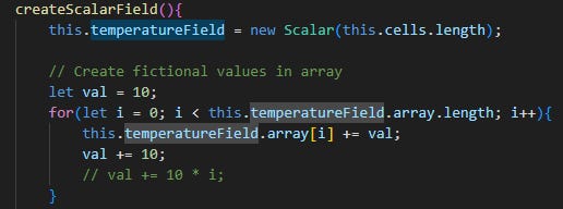
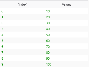
This is our scalar temperature field.
Each cell, from index 0 to 9 (or 1 – 10) has a value associated with it.
Here’s the same set of cells with a normalised colour scale applied, based on the temperature value in it:

If this was a vector field, I’d have both the magnitude and direction stored at each cell location. But we’re not dealing with this just yet.
Yes, these are fictional temperature values.
But we now have enough to calculate the change in temperature values between cells – or in other words, the temperature gradient.
The rate of change.
Mathematically, this is known as a spatial gradient.
Read as the slope of a curve that is plotting the change of temperature…
It depends directly on both the center distances and the actual scalar values present.
I manipulated the values and saw this pattern:
-
Values are the same / constant across cells i.e. all 10.
Gradient is 0.
-
Values increase linearly (as shown in table above).
Gradient is greater than 0 but remains the same.
-
Values increase in a non-linear way i.e. 10, 30, 65 etc…
Gradient is greater than 0 and increases cell to cell.
Hopefully you can appreciate that more cells, a smaller central distance, larger values etc. all change how the fluid behaves, even from this simple exercise.
Faces are the gates of the cell.
Considering the X-direction only in our 1D model, each cell has 2 faces through which heat can flow, in or out.
Before we can calculate this, I construct the faces as separate objects in my code so it’s clear what they hold and how they are used in calculations.
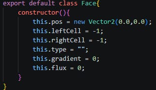
The most important thing to note is that a face has a record of its location and the neighbouring cells it sits in-between.
Internal faces have 2 cells adjacent to each other, while boundary faces will only have 1 cell.
A first experiment in computational fluid dynamics.
As a first experiment I calculated the heat flux by calculating the temperature gradient and the simple Fourier’s law for heat transfer.
Take a look at this short screen recording to inspect the results:
The gradient is consistent for the reason explained above.
We have a negative heat flux indicating the heat transfer direction is going from right to left, or from hot to cold, as it should be!
Watch me talk through the implementation of this in episode #03 on my YouTube channel:
I intentionally wrote all of this code by hand – I prefer to keep things as simple and clear as possible so you can follow and manipulate it with ease.
Have a great week!
Nasser
